2. Accessing Data
Damian Trilling and Penny Sheets
This notebook is meant to show you different ways of accessing data. Data can be available as (a) local files (on your computer), (b) remote files (somewhere else), or (c) APIs (application programming interfaces). We will show you ways for dealing with all of these.
But before we do that, we need to import some modules into Jupyter that will help us find and read data. You already know our basic module, pandas. Let’s import it again just in case your computer cleared it during the break (or in case you’re doing this notebook again separately, after class).
Importing Modules
It is a good custom to import all modules that you need at the beginning of your notebook. We’ll explain in the lesson (or in subsequent weeks) what these modules do.
import pandas as pd
from pprint import pprint
import json
import matplotlib.pyplot as plt
from collections import Counter
import requests
import seaborn as sns
%matplotlib inline
CSV files
Remember what we did in the first part of class today, working with that Iris dataset? We used pandas to read a CSV file directly from the web and gave its descriptive statistics.
iris = pd.read_csv('https://raw.githubusercontent.com/mwaskom/seaborn-data/master/iris.csv')
iris
| sepal_length | sepal_width | petal_length | petal_width | species | |
|---|---|---|---|---|---|
| 0 | 5.1 | 3.5 | 1.4 | 0.2 | setosa |
| 1 | 4.9 | 3.0 | 1.4 | 0.2 | setosa |
| 2 | 4.7 | 3.2 | 1.3 | 0.2 | setosa |
| 3 | 4.6 | 3.1 | 1.5 | 0.2 | setosa |
| 4 | 5.0 | 3.6 | 1.4 | 0.2 | setosa |
| ... | ... | ... | ... | ... | ... |
| 145 | 6.7 | 3.0 | 5.2 | 2.3 | virginica |
| 146 | 6.3 | 2.5 | 5.0 | 1.9 | virginica |
| 147 | 6.5 | 3.0 | 5.2 | 2.0 | virginica |
| 148 | 6.2 | 3.4 | 5.4 | 2.3 | virginica |
| 149 | 5.9 | 3.0 | 5.1 | 1.8 | virginica |
150 rows × 5 columns
iris.describe()
| sepal_length | sepal_width | petal_length | petal_width | |
|---|---|---|---|---|
| count | 150.000000 | 150.000000 | 150.000000 | 150.000000 |
| mean | 5.843333 | 3.057333 | 3.758000 | 1.199333 |
| std | 0.828066 | 0.435866 | 1.765298 | 0.762238 |
| min | 4.300000 | 2.000000 | 1.000000 | 0.100000 |
| 25% | 5.100000 | 2.800000 | 1.600000 | 0.300000 |
| 50% | 5.800000 | 3.000000 | 4.350000 | 1.300000 |
| 75% | 6.400000 | 3.300000 | 5.100000 | 1.800000 |
| max | 7.900000 | 4.400000 | 6.900000 | 2.500000 |
If we want to, we could also plot a histogram:
iris.sepal_length.hist()
<AxesSubplot:>
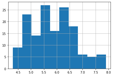
Let’s say you want to configure that histogram differently, or get axis lables, etc. Use the help menu to see how to do that:
iris.sepal_length.hist?
Signature:
iris.sepal_length.hist(
    by=None,
    ax=None,
    grid: 'bool' = True,
    xlabelsize: 'int | None' = None,
    xrot: 'float | None' = None,
    ylabelsize: 'int | None' = None,
    yrot: 'float | None' = None,
    figsize: 'tuple[int, int] | None' = None,
    bins: 'int | Sequence[int]' = 10,
    backend: 'str | None' = None,
    legend: 'bool' = False,
    **kwargs,
)
Docstring:
Draw histogram of the input series using matplotlib.

Parameters
----------
by : object, optional
    If passed, then used to form histograms for separate groups.
ax : matplotlib axis object
    If not passed, uses gca().
grid : bool, default True
    Whether to show axis grid lines.
xlabelsize : int, default None
    If specified changes the x-axis label size.
xrot : float, default None
    Rotation of x axis labels.
ylabelsize : int, default None
    If specified changes the y-axis label size.
yrot : float, default None
    Rotation of y axis labels.
figsize : tuple, default None
    Figure size in inches by default.
bins : int or sequence, default 10
    Number of histogram bins to be used. If an integer is given, bins + 1
    bin edges are calculated and returned. If bins is a sequence, gives
    bin edges, including left edge of first bin and right edge of last
    bin. In this case, bins is returned unmodified.
backend : str, default None
    Backend to use instead of the backend specified in the option
    ``plotting.backend``. For instance, 'matplotlib'. Alternatively, to
    specify the ``plotting.backend`` for the whole session, set
    ``pd.options.plotting.backend``.

    .. versionadded:: 1.0.0

legend : bool, default False
    Whether to show the legend.

    .. versionadded:: 1.1.0

**kwargs
    To be passed to the actual plotting function.

Returns
-------
matplotlib.AxesSubplot
    A histogram plot.

See Also
--------
matplotlib.axes.Axes.hist : Plot a histogram using matplotlib.
File:      ~/opt/anaconda3/envs/dj21/lib/python3.7/site-packages/pandas/plotting/_core.py
Type:      method
Downloading data
Probably, if you really want to analyze a dataset, you want to store it locally (=on your computer). Let’s download a file with some stock exchange ratings: https://raw.githubusercontent.com/damian0604/bdaca/master/ipynb/stock.csv
Download it (file-save as or right-clicking) as “all file types” (or .csv); be sure that the extension is correct. Be sure to save it IN THE SAME FOLDER as this jupyter notebook. (Otherwise jupyter won’t find it.)
Note!!! Not all CSV files are the same…
CSV stands for Comma Seperated Value, which indicates that it consists of values (columns) seperated by commas. Just open a CSV file in an editor like Notepad or TextEdit instead of in Excel to understand what we mean.
Unfortunately, there are many different dialects. For instance, sometimes, a semicolon or a tab is used instead of a comma; sometimes, the first line of a CSV file contains column headers, sometimes not) You can indicate these type of details yourself if pandas doesn’t guess correctly.
Pay special attention when opening a CSV file with Excel: Excel changes the formatting! For instance, it can happen that you open a file that uses commas as seperators in Excel, and when you save it, it suddenly uses semicolons instead.
Another reason not to open your files in Excel first: Excel often creates a strange ‘encoding’ of the characters that causes problems here. This is why we work just with the raw .csv file if possible. If you are getting an encoding error, the first step is to re-download the data and do NOT open it in excel (even by mistake, by double-clicking on it).
We can then open it in the same way as we did before by providing its filename:
# stockdata = pd.read_csv('stock.csv') # if you downloaded and saved it locally
stockdata = pd.read_csv('https://raw.githubusercontent.com/damian0604/bdaca/master/ipynb/stock.csv') # when reading directly from source (online)
Let’s have a look…
stockdata
| Date | Open | High | Low | Close | Volume | Adj Close | |
|---|---|---|---|---|---|---|---|
| 0 | 2016-01-01 | 21.095 | 21.095 | 21.095 | 21.095 | 0 | 20.6742 |
| 1 | 2015-12-31 | 21.135 | 21.140 | 20.915 | 21.095 | 1680700 | 20.6742 |
| 2 | 2015-12-30 | 21.330 | 21.375 | 21.110 | 21.185 | 5476800 | 20.7624 |
| 3 | 2015-12-29 | 21.000 | 21.410 | 20.995 | 21.325 | 6261600 | 20.8996 |
| 4 | 2015-12-28 | 21.440 | 21.450 | 20.705 | 20.880 | 5168400 | 20.4635 |
| ... | ... | ... | ... | ... | ... | ... | ... |
| 518 | 2014-01-07 | 25.810 | 26.065 | 25.720 | 26.030 | 5330200 | 22.9539 |
| 519 | 2014-01-06 | 26.015 | 26.030 | 25.790 | 25.810 | 4775300 | 22.7599 |
| 520 | 2014-01-03 | 26.000 | 26.195 | 25.875 | 26.065 | 4298100 | 22.9848 |
| 521 | 2014-01-02 | 25.985 | 26.130 | 25.855 | 25.920 | 5113500 | 22.8569 |
| 522 | 2014-01-01 | 25.905 | 25.905 | 25.905 | 25.905 | 0 | 22.8437 |
523 rows × 7 columns
The lefthand column here–called the index–gives you numbers in this case; these are simply the case numbers for each ‘row’ in the dataset; they may or may not have any meaning on their own, depending on the dataset. You can also - later in this notebook and later in subsequent weeks - learn how to change these numbers or assign a different column to be the index.
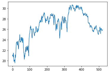
Because this data seems to be ordered by date in some way, it might be interesting to explore it by making a plot. In this case the plot is different than the histogram; it’s not about frequencies of specific values, but rather a plot of all the cases at their value of ‘low’.
We are using a method here called ‘plot’, provided by pandas.
stockdata['Low'].plot()
<AxesSubplot:>
Trouble with your CSV files?
For more info on how to format your ‘read_csv’ commands, or if you’re running into problems related to the comma-versus-tab-versus-semicolon issue, look at the help function:
pd.read_csv?
Signature:
pd.read_csv(
    filepath_or_buffer: 'FilePathOrBuffer',
    sep=<no_default>,
    delimiter=None,
    header='infer',
    names=<no_default>,
    index_col=None,
    usecols=None,
    squeeze=False,
    prefix=<no_default>,
    mangle_dupe_cols=True,
    dtype: 'DtypeArg | None' = None,
    engine=None,
    converters=None,
    true_values=None,
    false_values=None,
    skipinitialspace=False,
    skiprows=None,
    skipfooter=0,
    nrows=None,
    na_values=None,
    keep_default_na=True,
    na_filter=True,
    verbose=False,
    skip_blank_lines=True,
    parse_dates=False,
    infer_datetime_format=False,
    keep_date_col=False,
    date_parser=None,
    dayfirst=False,
    cache_dates=True,
    iterator=False,
    chunksize=None,
    compression='infer',
    thousands=None,
    decimal: 'str' = '.',
    lineterminator=None,
    quotechar='"',
    quoting=0,
    doublequote=True,
    escapechar=None,
    comment=None,
    encoding=None,
    encoding_errors: 'str | None' = 'strict',
    dialect=None,
    error_bad_lines=None,
    warn_bad_lines=None,
    on_bad_lines=None,
    delim_whitespace=False,
    low_memory=True,
    memory_map=False,
    float_precision=None,
    storage_options: 'StorageOptions' = None,
)
Docstring:
Read a comma-separated values (csv) file into DataFrame.

Also supports optionally iterating or breaking of the file
into chunks.

Additional help can be found in the online docs for
`IO Tools <https://pandas.pydata.org/pandas-docs/stable/user_guide/io.html>`_.

Parameters
----------
filepath_or_buffer : str, path object or file-like object
    Any valid string path is acceptable. The string could be a URL. Valid
    URL schemes include http, ftp, s3, gs, and file. For file URLs, a host is
    expected. A local file could be: file://localhost/path/to/table.csv.

    If you want to pass in a path object, pandas accepts any ``os.PathLike``.

    By file-like object, we refer to objects with a ``read()`` method, such as
    a file handle (e.g. via builtin ``open`` function) or ``StringIO``.
sep : str, default ','
    Delimiter to use. If sep is None, the C engine cannot automatically detect
    the separator, but the Python parsing engine can, meaning the latter will
    be used and automatically detect the separator by Python's builtin sniffer
    tool, ``csv.Sniffer``. In addition, separators longer than 1 character and
    different from ``'\s+'`` will be interpreted as regular expressions and
    will also force the use of the Python parsing engine. Note that regex
    delimiters are prone to ignoring quoted data. Regex example: ``'\r\t'``.
delimiter : str, default ``None``
    Alias for sep.
header : int, list of int, default 'infer'
    Row number(s) to use as the column names, and the start of the
    data.  Default behavior is to infer the column names: if no names
    are passed the behavior is identical to ``header=0`` and column
    names are inferred from the first line of the file, if column
    names are passed explicitly then the behavior is identical to
    ``header=None``. Explicitly pass ``header=0`` to be able to
    replace existing names. The header can be a list of integers that
    specify row locations for a multi-index on the columns
    e.g. [0,1,3]. Intervening rows that are not specified will be
    skipped (e.g. 2 in this example is skipped). Note that this
    parameter ignores commented lines and empty lines if
    ``skip_blank_lines=True``, so ``header=0`` denotes the first line of
    data rather than the first line of the file.
names : array-like, optional
    List of column names to use. If the file contains a header row,
    then you should explicitly pass ``header=0`` to override the column names.
    Duplicates in this list are not allowed.
index_col : int, str, sequence of int / str, or False, default ``None``
  Column(s) to use as the row labels of the ``DataFrame``, either given as
  string name or column index. If a sequence of int / str is given, a
  MultiIndex is used.

  Note: ``index_col=False`` can be used to force pandas to *not* use the first
  column as the index, e.g. when you have a malformed file with delimiters at
  the end of each line.
usecols : list-like or callable, optional
    Return a subset of the columns. If list-like, all elements must either
    be positional (i.e. integer indices into the document columns) or strings
    that correspond to column names provided either by the user in `names` or
    inferred from the document header row(s). For example, a valid list-like
    `usecols` parameter would be ``[0, 1, 2]`` or ``['foo', 'bar', 'baz']``.
    Element order is ignored, so ``usecols=[0, 1]`` is the same as ``[1, 0]``.
    To instantiate a DataFrame from ``data`` with element order preserved use
    ``pd.read_csv(data, usecols=['foo', 'bar'])[['foo', 'bar']]`` for columns
    in ``['foo', 'bar']`` order or
    ``pd.read_csv(data, usecols=['foo', 'bar'])[['bar', 'foo']]``
    for ``['bar', 'foo']`` order.

    If callable, the callable function will be evaluated against the column
    names, returning names where the callable function evaluates to True. An
    example of a valid callable argument would be ``lambda x: x.upper() in
    ['AAA', 'BBB', 'DDD']``. Using this parameter results in much faster
    parsing time and lower memory usage.
squeeze : bool, default False
    If the parsed data only contains one column then return a Series.
prefix : str, optional
    Prefix to add to column numbers when no header, e.g. 'X' for X0, X1, ...
mangle_dupe_cols : bool, default True
    Duplicate columns will be specified as 'X', 'X.1', ...'X.N', rather than
    'X'...'X'. Passing in False will cause data to be overwritten if there
    are duplicate names in the columns.
dtype : Type name or dict of column -> type, optional
    Data type for data or columns. E.g. {'a': np.float64, 'b': np.int32,
    'c': 'Int64'}
    Use `str` or `object` together with suitable `na_values` settings
    to preserve and not interpret dtype.
    If converters are specified, they will be applied INSTEAD
    of dtype conversion.
engine : {'c', 'python'}, optional
    Parser engine to use. The C engine is faster while the python engine is
    currently more feature-complete.
converters : dict, optional
    Dict of functions for converting values in certain columns. Keys can either
    be integers or column labels.
true_values : list, optional
    Values to consider as True.
false_values : list, optional
    Values to consider as False.
skipinitialspace : bool, default False
    Skip spaces after delimiter.
skiprows : list-like, int or callable, optional
    Line numbers to skip (0-indexed) or number of lines to skip (int)
    at the start of the file.

    If callable, the callable function will be evaluated against the row
    indices, returning True if the row should be skipped and False otherwise.
    An example of a valid callable argument would be ``lambda x: x in [0, 2]``.
skipfooter : int, default 0
    Number of lines at bottom of file to skip (Unsupported with engine='c').
nrows : int, optional
    Number of rows of file to read. Useful for reading pieces of large files.
na_values : scalar, str, list-like, or dict, optional
    Additional strings to recognize as NA/NaN. If dict passed, specific
    per-column NA values.  By default the following values are interpreted as
    NaN: '', '#N/A', '#N/A N/A', '#NA', '-1.#IND', '-1.#QNAN', '-NaN', '-nan',
    '1.#IND', '1.#QNAN', '<NA>', 'N/A', 'NA', 'NULL', 'NaN', 'n/a',
    'nan', 'null'.
keep_default_na : bool, default True
    Whether or not to include the default NaN values when parsing the data.
    Depending on whether `na_values` is passed in, the behavior is as follows:

    * If `keep_default_na` is True, and `na_values` are specified, `na_values`
      is appended to the default NaN values used for parsing.
    * If `keep_default_na` is True, and `na_values` are not specified, only
      the default NaN values are used for parsing.
    * If `keep_default_na` is False, and `na_values` are specified, only
      the NaN values specified `na_values` are used for parsing.
    * If `keep_default_na` is False, and `na_values` are not specified, no
      strings will be parsed as NaN.

    Note that if `na_filter` is passed in as False, the `keep_default_na` and
    `na_values` parameters will be ignored.
na_filter : bool, default True
    Detect missing value markers (empty strings and the value of na_values). In
    data without any NAs, passing na_filter=False can improve the performance
    of reading a large file.
verbose : bool, default False
    Indicate number of NA values placed in non-numeric columns.
skip_blank_lines : bool, default True
    If True, skip over blank lines rather than interpreting as NaN values.
parse_dates : bool or list of int or names or list of lists or dict, default False
    The behavior is as follows:

    * boolean. If True -> try parsing the index.
    * list of int or names. e.g. If [1, 2, 3] -> try parsing columns 1, 2, 3
      each as a separate date column.
    * list of lists. e.g.  If [[1, 3]] -> combine columns 1 and 3 and parse as
      a single date column.
    * dict, e.g. {'foo' : [1, 3]} -> parse columns 1, 3 as date and call
      result 'foo'

    If a column or index cannot be represented as an array of datetimes,
    say because of an unparsable value or a mixture of timezones, the column
    or index will be returned unaltered as an object data type. For
    non-standard datetime parsing, use ``pd.to_datetime`` after
    ``pd.read_csv``. To parse an index or column with a mixture of timezones,
    specify ``date_parser`` to be a partially-applied
    :func:`pandas.to_datetime` with ``utc=True``. See
    :ref:`io.csv.mixed_timezones` for more.

    Note: A fast-path exists for iso8601-formatted dates.
infer_datetime_format : bool, default False
    If True and `parse_dates` is enabled, pandas will attempt to infer the
    format of the datetime strings in the columns, and if it can be inferred,
    switch to a faster method of parsing them. In some cases this can increase
    the parsing speed by 5-10x.
keep_date_col : bool, default False
    If True and `parse_dates` specifies combining multiple columns then
    keep the original columns.
date_parser : function, optional
    Function to use for converting a sequence of string columns to an array of
    datetime instances. The default uses ``dateutil.parser.parser`` to do the
    conversion. Pandas will try to call `date_parser` in three different ways,
    advancing to the next if an exception occurs: 1) Pass one or more arrays
    (as defined by `parse_dates`) as arguments; 2) concatenate (row-wise) the
    string values from the columns defined by `parse_dates` into a single array
    and pass that; and 3) call `date_parser` once for each row using one or
    more strings (corresponding to the columns defined by `parse_dates`) as
    arguments.
dayfirst : bool, default False
    DD/MM format dates, international and European format.
cache_dates : bool, default True
    If True, use a cache of unique, converted dates to apply the datetime
    conversion. May produce significant speed-up when parsing duplicate
    date strings, especially ones with timezone offsets.

    .. versionadded:: 0.25.0
iterator : bool, default False
    Return TextFileReader object for iteration or getting chunks with
    ``get_chunk()``.

    .. versionchanged:: 1.2

       ``TextFileReader`` is a context manager.
chunksize : int, optional
    Return TextFileReader object for iteration.
    See the `IO Tools docs
    <https://pandas.pydata.org/pandas-docs/stable/io.html#io-chunking>`_
    for more information on ``iterator`` and ``chunksize``.

    .. versionchanged:: 1.2

       ``TextFileReader`` is a context manager.
compression : {'infer', 'gzip', 'bz2', 'zip', 'xz', None}, default 'infer'
    For on-the-fly decompression of on-disk data. If 'infer' and
    `filepath_or_buffer` is path-like, then detect compression from the
    following extensions: '.gz', '.bz2', '.zip', or '.xz' (otherwise no
    decompression). If using 'zip', the ZIP file must contain only one data
    file to be read in. Set to None for no decompression.
thousands : str, optional
    Thousands separator.
decimal : str, default '.'
    Character to recognize as decimal point (e.g. use ',' for European data).
lineterminator : str (length 1), optional
    Character to break file into lines. Only valid with C parser.
quotechar : str (length 1), optional
    The character used to denote the start and end of a quoted item. Quoted
    items can include the delimiter and it will be ignored.
quoting : int or csv.QUOTE_* instance, default 0
    Control field quoting behavior per ``csv.QUOTE_*`` constants. Use one of
    QUOTE_MINIMAL (0), QUOTE_ALL (1), QUOTE_NONNUMERIC (2) or QUOTE_NONE (3).
doublequote : bool, default ``True``
   When quotechar is specified and quoting is not ``QUOTE_NONE``, indicate
   whether or not to interpret two consecutive quotechar elements INSIDE a
   field as a single ``quotechar`` element.
escapechar : str (length 1), optional
    One-character string used to escape other characters.
comment : str, optional
    Indicates remainder of line should not be parsed. If found at the beginning
    of a line, the line will be ignored altogether. This parameter must be a
    single character. Like empty lines (as long as ``skip_blank_lines=True``),
    fully commented lines are ignored by the parameter `header` but not by
    `skiprows`. For example, if ``comment='#'``, parsing
    ``#empty\na,b,c\n1,2,3`` with ``header=0`` will result in 'a,b,c' being
    treated as the header.
encoding : str, optional
    Encoding to use for UTF when reading/writing (ex. 'utf-8'). `List of Python
    standard encodings
    <https://docs.python.org/3/library/codecs.html#standard-encodings>`_ .

    .. versionchanged:: 1.2

       When ``encoding`` is ``None``, ``errors="replace"`` is passed to
       ``open()``. Otherwise, ``errors="strict"`` is passed to ``open()``.
       This behavior was previously only the case for ``engine="python"``.

    .. versionchanged:: 1.3.0

       ``encoding_errors`` is a new argument. ``encoding`` has no longer an
       influence on how encoding errors are handled.

encoding_errors : str, optional, default "strict"
    How encoding errors are treated. `List of possible values
    <https://docs.python.org/3/library/codecs.html#error-handlers>`_ .

    .. versionadded:: 1.3.0

dialect : str or csv.Dialect, optional
    If provided, this parameter will override values (default or not) for the
    following parameters: `delimiter`, `doublequote`, `escapechar`,
    `skipinitialspace`, `quotechar`, and `quoting`. If it is necessary to
    override values, a ParserWarning will be issued. See csv.Dialect
    documentation for more details.
error_bad_lines : bool, default ``None``
    Lines with too many fields (e.g. a csv line with too many commas) will by
    default cause an exception to be raised, and no DataFrame will be returned.
    If False, then these "bad lines" will be dropped from the DataFrame that is
    returned.

    .. deprecated:: 1.3.0
       The ``on_bad_lines`` parameter should be used instead to specify behavior upon
       encountering a bad line instead.
warn_bad_lines : bool, default ``None``
    If error_bad_lines is False, and warn_bad_lines is True, a warning for each
    "bad line" will be output.

    .. deprecated:: 1.3.0
       The ``on_bad_lines`` parameter should be used instead to specify behavior upon
       encountering a bad line instead.
on_bad_lines : {'error', 'warn', 'skip'}, default 'error'
    Specifies what to do upon encountering a bad line (a line with too many fields).
    Allowed values are :

        - 'error', raise an Exception when a bad line is encountered.
        - 'warn', raise a warning when a bad line is encountered and skip that line.
        - 'skip', skip bad lines without raising or warning when they are encountered.

    .. versionadded:: 1.3.0

delim_whitespace : bool, default False
    Specifies whether or not whitespace (e.g. ``' '`` or ``'    '``) will be
    used as the sep. Equivalent to setting ``sep='\s+'``. If this option
    is set to True, nothing should be passed in for the ``delimiter``
    parameter.
low_memory : bool, default True
    Internally process the file in chunks, resulting in lower memory use
    while parsing, but possibly mixed type inference.  To ensure no mixed
    types either set False, or specify the type with the `dtype` parameter.
    Note that the entire file is read into a single DataFrame regardless,
    use the `chunksize` or `iterator` parameter to return the data in chunks.
    (Only valid with C parser).
memory_map : bool, default False
    If a filepath is provided for `filepath_or_buffer`, map the file object
    directly onto memory and access the data directly from there. Using this
    option can improve performance because there is no longer any I/O overhead.
float_precision : str, optional
    Specifies which converter the C engine should use for floating-point
    values. The options are ``None`` or 'high' for the ordinary converter,
    'legacy' for the original lower precision pandas converter, and
    'round_trip' for the round-trip converter.

    .. versionchanged:: 1.2

storage_options : dict, optional
    Extra options that make sense for a particular storage connection, e.g.
    host, port, username, password, etc. For HTTP(S) URLs the key-value pairs
    are forwarded to ``urllib`` as header options. For other URLs (e.g.
    starting with "s3://", and "gcs://") the key-value pairs are forwarded to
    ``fsspec``. Please see ``fsspec`` and ``urllib`` for more details.

    .. versionadded:: 1.2

Returns
-------
DataFrame or TextParser
    A comma-separated values (csv) file is returned as two-dimensional
    data structure with labeled axes.

See Also
--------
DataFrame.to_csv : Write DataFrame to a comma-separated values (csv) file.
read_csv : Read a comma-separated values (csv) file into DataFrame.
read_fwf : Read a table of fixed-width formatted lines into DataFrame.

Examples
--------
>>> pd.read_csv('data.csv')  # doctest: +SKIP
File:      ~/opt/anaconda3/envs/dj21/lib/python3.7/site-packages/pandas/io/parsers/readers.py
Type:      function
What if the data isn’t in .csv format, but is online?
There is actually a very simple, brilliant, scraping tool that allows you to grab content from tables online and turn that into a csv file. Then you can use the tools we just used to analyze the csv file (including saving it to your computer and importing it into jupyter for analysis). The tool is called read_html and allows you to basically put in any website URL and scrape the tables from it. It probably won’t work with all websites (and probably not everything it scrapes is relevant/useful to you), but, it is really handy when it does work. Let’s look, for example, at wikipedia’s page involving the premier Dutch football league.
First, load the URL into your browswer in another tab to look at the original page.
alltables = pd.read_html('https://en.wikipedia.org/wiki/Eredivisie')
Look at the following code carefully to see what we’re doing here. We’re introducing a new method (“format”) which works for any string; this fills in a value between curly brackets. We also are using function we already know from the first part of today’s lesson: “len”.
print('We have downloaded {} tables'.format(len(alltables)))
We have downloaded 19 tables
Here is another, perhaps simpler way to do this, but also less versatile if you want to do fancier stuff someday.
The point here is that there are multiple ways to do many things in python; we just want you to master one way and know why it’s useful to you.
print('We have downloaded', len(alltables), 'tables.')
We have downloaded 19 tables.
Let’s look at, say, the third table in this set.
alltables[2]
#why is this not 3? It is because python uses 0-based indexing, which means that data, values, rows, and items
#in lists, which you've seen in your coding tutorials, all start at 0. So the first object in a list or index
#is always in position "0", and the second in position "1", and so on.  In this case, to get the 3rd table in
#this new little set of tables, we have to specify "2" rather than "3".
| Club | Winner | Runner-up | Winning years | |
|---|---|---|---|---|
| 0 | Ajax | 35 | 23 | 1917–18, 1918–19, 1930–31, 1931–32, 1933–34, 1... |
| 1 | PSV Eindhoven | 24 | 14 | 1928–29, 1934–35, 1950–51, 1962–63, 1974–75, 1... |
| 2 | Feyenoord | 15 | 21 | 1923–24, 1927–28, 1935–36, 1937–38, 1939–40, 1... |
| 3 | HVV Den Haag | 10 | 1 | 1890–91, 1895–96, 1899–1900, 1900–01, 1901–02,... |
| 4 | Sparta Rotterdam | 6 | – | 1908–09, 1910–11, 1911–12, 1912–13, 1914–15, 1... |
| 5 | RAP | 5 | 3 | 1891–92, 1893–94, 1896–97, 1897–98, 1898–99 |
| 6 | Go Ahead Eagles | 4 | 5 | 1916–17, 1921–22, 1929–30, 1932–33 |
| 7 | Koninklijke HFC | 3 | 3 | 1889–90, 1892–93, 1894–95 |
| 8 | Willem II | 3 | 1 | 1915–16, 1951–52, 1954–55 |
| 9 | HBS Craeyenhout | 3 | – | 1903–04, 1905–06, 1924–25 |
| 10 | AZ | 2 | 3 | 1980–81, 2008–09 |
| 11 | Heracles Almelo | 2 | 1 | 1926–27, 1940–41 |
| 12 | ADO Den Haag | 2 | – | 1941–42, 1942–43 |
| 13 | RCH | 2 | – | 1922–23, 1952–53 |
| 14 | NAC Breda | 1 | 4 | 1920–21 |
| 15 | FC Twente | 1 | 3 | 2009–10 |
| 16 | DWS | 1 | 3 | 1963–64 |
| 17 | Roda JC Kerkrade* | 1 | 2 | 1955–56 |
| 18 | Be Quick | 1 | 2 | 1919–20 |
| 19 | FC Eindhoven | 1 | 2 | 1953–54 |
| 20 | SC Enschede | 1 | 1 | 1925–26 |
| 21 | DOS | 1 | 1 | 1957–58 |
| 22 | FC Den Bosch | 1 | 1 | 1947–48 |
| 23 | De Volewijckers | 1 | – | 1943–44 |
| 24 | HFC Haarlem | 1 | – | 1945–46 |
| 25 | Limburgia | 1 | – | 1949–50 |
| 26 | SVV | 1 | – | 1948–49 |
| 27 | Quick Den Haag | 1 | – | 1907–08 |
| 28 | VV Concordia | 1 | – | 1888–89 |
Now we can save this table to a csv file, which we will call ‘test’:
alltables[2].to_csv('test.csv')
Now, see if you can go back and read in this test.csv file, have a look at the dataset.
If we had more time, we would try to figure out how to rename the columns, and play around with plotting the number of times each team won, for example. (Try this at home, and see if you can do it! Using the read help command from earlier should help you figure out how to rename columns…or when in doubt, just search online for help!)
JSON files
Another type of file we frequently encounter online is the so-called “jason” file - aka, JSON. JSON files allow for nested data structures–like databases.
JSON is (basically) the same as a collection of Python dicts (dictionaries–we haven’t talked about these yet in class, but you did learn about this in your coding tutorials. As a reminder, dicts are collections of key:value pairs, which means you have a category of something (key) and values within it (values)). I’ll explain this in class more. Bottom line: it’s very easy to look up things by their key, but not by their values. So, knowing our way around these dicts and how they are nested within one another - in a json file - is important.
Let’s download such a file and store it in the same directory as your jupyter notebook. Download https://open.data.amsterdam.nl/EtenDrinken.json .
First, see what happens if you load this link in your browser. You can get a feel for the structure of the dataset, if your browser is relatively fancy.
Next: we could use pandas to put the JSON file into a table (see next command) – but as you see, because the data is nested, we still have dicts within some of the cells:
Note: The location (often called path) where you stored the file is important to remember when you load the data into your notebook. I have saved the json file to a folder called datasets, which is located one folder ‘above’ the current folder where our notebook reside in. So, I have to tell Python to go back one folder (‘../’), then into the datasets folder (datasets/), and from there open the file ‘EtenDrinken.json’. If you stored the datafile in the same folder as your notebook is in, you can just load it by providing the file name!
Where am I? If you are unsure where your notebook is running from, simply use the following cell magic to get the path to your current notebook:
!pwd
/Users/fhopp/Library/Mobile Documents/com~apple~CloudDocs/FRH/Science/ASCoR/Teaching/data_journalism/21/book_dj/content
pd.read_json('EtenDrinken.json')
# pd.read_json('EtenDrinken.json') if your file is in the same folder as this notebook
| trcid | title | details | types | location | urls | media | dates | lastupdated | eigenschappen | |
|---|---|---|---|---|---|---|---|---|---|---|
| 0 | 853c93aa-4599-41ad-9d79-638902925dc9 | Eetsalon van Dobben B.V. | {'de': {'language': 'de', 'title': 'Eetsalon v... | [{'type': '', 'catid': '3.2.1'}] | {'name': '', 'city': 'AMSTERDAM', 'adress': 'K... | [http://www.eetsalonvandobben.nl, http://www.f... | [{'url': 'https://media.iamsterdam.com/ndtrc/I... | {'startdate': '27-01-2011', 'enddate': ''} | 2016-09-19 13:58:20 | {'3.6': {'Catid': '3.6', 'Value': 'True', 'Cat... |
| 1 | a9dca5a2-aaeb-4d11-9025-f8ab29d6e042 | Eetsalon van Dobben de Pijp | {'de': {'language': 'de', 'title': 'Eetsalon v... | [{'type': '', 'catid': '3.2.1'}] | {'name': 'Eetsalon van Dobben de Pijp', 'city'... | [] | [{'url': 'https://media.iamsterdam.com/ndtrc/I... | [] | 2016-04-03 10:40:22 | {'3.6': {'Catid': '3.6', 'Value': 'True', 'Cat... |
| 2 | 2ed5f9de-2850-4bcd-affe-4b19b4144906 | Cora Delicatessen & Broodjes | {'de': {'language': 'de', 'title': 'Cora Delic... | [{'type': '', 'catid': '3.2.1'}] | {'name': 'Cora Delicatessen & Broodjes', 'city... | [http://www.cora-broodjes.nl/] | [{'url': 'https://media.iamsterdam.com/ndtrc/I... | [] | 2015-06-23 10:08:59 | [] |
| 3 | 54d3daf4-610d-4328-a657-65a05c047eb9 | Jonk Haringhandel | {'de': {'language': 'de', 'title': 'Jonk Harin... | [{'type': '', 'catid': '3.2.1'}] | {'name': 'Jonk Haringhandel', 'city': 'AMSTERD... | [] | [{'url': 'https://media.iamsterdam.com/ndtrc/I... | [] | 2017-01-17 17:17:36 | {'3.6': {'Catid': '3.6', 'Value': 'True', 'Cat... |
| 4 | 41de3334-b0b2-43be-b226-b39b106d96f6 | Vlaamsch Broodhuys | {'de': {'language': 'de', 'title': 'Vlaamsch B... | [{'type': '', 'catid': '3.2.1'}] | {'name': 'Vlaamsch Broodhuys', 'city': 'AMSTER... | [http://www.vlaamschbroodhuys.nl/index.php/gb] | [{'url': 'https://media.iamsterdam.com/ndtrc/I... | {'startdate': '08-08-2013', 'enddate': ''} | 2017-01-18 14:56:34 | {'42.2': {'Catid': '42.2', 'Value': {}, 'Categ... |
| ... | ... | ... | ... | ... | ... | ... | ... | ... | ... | ... |
| 767 | 07c43eb7-dc3f-4643-933e-6d8c7cfc39af | Strandpaviljoen Timboektoe | {'de': {'language': 'de', 'title': 'Strandbar ... | [{'type': '', 'catid': '3.1.5'}] | {'name': 'Strandpaviljoen Timboektoe', 'city':... | [http://www.timboektoe.org, http://www.faceboo... | [{'url': 'https://media.ndtrc.nl/Images/07/07c... | [] | 2017-07-25 14:04:21 | {'34.2': {'Catid': '34.2', 'Value': {}, 'Categ... |
| 768 | 680a178e-0941-4db0-bb6a-120710536630 | Paviljoen Zeezicht | {'de': {'language': 'de', 'title': 'Strandbar ... | [{'type': '', 'catid': '3.1.5'}] | {'name': 'Paviljoen Zeezicht', 'city': 'IJMUID... | [http://www.paviljoenzeezicht.nl] | [{'url': 'https://media.ndtrc.nl/Images/201102... | [] | 2017-07-26 12:15:29 | {'34.2': {'Catid': '34.2', 'Value': {}, 'Categ... |
| 769 | eaca1623-baef-4e4b-9fcb-c19de652e042 | Paviljoen Nova Zembla | {'de': {'language': 'de', 'title': 'Strandbar ... | [{'type': '', 'catid': '3.1.5'}] | {'name': '', 'city': 'IJMUIDEN', 'adress': 'Ke... | [http://www.paviljoennovazembla.nl/] | [{'url': 'https://media.ndtrc.nl/Images/201202... | [] | 2017-07-26 12:14:43 | {'10.11': {'Catid': '10.11', 'Value': 'True', ... |
| 770 | b75d4392-ae17-4820-a62a-1ead2a604ab2 | Beach Inn | {'de': {'language': 'de', 'title': 'Beach Inn'... | [{'type': '', 'catid': '3.1.5'}] | {'name': 'Beach Inn', 'city': 'IJMUIDEN', 'adr... | [http://www.beachinn-events.nl/, http://www.fa... | [{'url': 'https://media.ndtrc.nl/Images/201303... | [] | 2017-07-26 12:13:07 | {'34.13': {'Catid': '34.13', 'Value': 'true'},... |
| 771 | 7e7be9d0-1391-4875-b284-ea93ea87e0dd | Paviljoen Noordzee | {'de': {'language': 'de', 'title': 'Strandbar ... | [{'type': '', 'catid': '3.1.5'}] | {'name': '', 'city': 'IJMUIDEN', 'adress': 'Ke... | [http://www.paviljoennoordzee.nl] | [{'url': 'https://media.ndtrc.nl/Images/201101... | [] | 2017-07-26 12:13:56 | {'34.1': {'Catid': '34.1', 'Value': {}, 'Categ... |
772 rows × 10 columns
Sometimes, pandas can be an easy solution for dealing with JSON files, but in this case, it doesn’t seem to be the best choice.
So, let’s read the JSON file into a list of dictionaries instead, since most of these columns seem to include dictionaries. We’re going to call it “eat”, this new list of dictionaries, because we know from the site this has something to do with eating and drinking.
eat = json.load(open('EtenDrinken.json'))
#note: nothing happens in terms of output for this command.
#but now it's in a format we can more easily explore in python.
Playing around with nested JSON data and extracting meaningful information
NOTE!! You don’t need to be able to do all of this already, but it’s mostly important that you try to understand the logic behind these various commands. We’ll review a lot of this later on when we get to analysis, anyway.
Let’s check what eat is and what is in there
type(eat)
list
len(eat)
772
Maybe let’s just look at the first restaurant
pprint(eat[0])
#pprint stands for 'pretty print'--it's not terribly pretty,
#but nicer than if you do just a plain old print (try it out!)
{'dates': {'enddate': '', 'startdate': '27-01-2011'},
 'details': {'de': {'calendarsummary': 'Mo -Mi : 10:00 - 21:00 Uhr\n'
                                       'Do : 10:00 - 01:00 Uhr\n'
                                       'Fr , Sa : 10:00 - 02:00 Uhr\n'
                                       'So : 10:30 - 20:00 Uhr.',
                    'language': 'de',
                    'longdescription': '',
                    'shortdescription': '',
                    'title': 'Eetsalon van Dobben B.V.'},
             'en': {'calendarsummary': 'Mo -We : 10:00 - 21:00 hour\n'
                                       'Th : 10:00 - 01:00 hour\n'
                                       'Fr , Sa : 10:00 - 02:00 hour\n'
                                       'Su: 10:30 - 20:00 hour.',
                    'language': 'en',
                    'longdescription': '',
                    'shortdescription': 'This typical Amsterdam deluxe '
                                        'lunchroom is the meeting place of '
                                        'artists, soccer players and many '
                                        'other locals. Its Van Dobben '
                                        'croquette is famed far beyond the '
                                        'city limits.',
                    'title': 'Eetsalon van Dobben B.V.'},
             'es': {'calendarsummary': 'Lu -Mi : 10:00 - 21:00 Hora\n'
                                       'Ju : 10:00 - 01:00 Hora\n'
                                       'Vi , Sa : 10:00 - 02:00 Hora\n'
                                       'Do : 10:30 - 20:00 Hora.',
                    'language': 'es',
                    'longdescription': '',
                    'shortdescription': '',
                    'title': 'Eetsalon van Dobben B.V.'},
             'fr': {'calendarsummary': 'Lu -Me : 10:00 - 21:00 heure\n'
                                       'Je : 10:00 - 01:00 heure\n'
                                       'Ve , Sa : 10:00 - 02:00 heure\n'
                                       'Di : 10:30 - 20:00 heure.',
                    'language': 'fr',
                    'longdescription': '',
                    'shortdescription': '',
                    'title': 'Eetsalon van Dobben B.V.'},
             'it': {'calendarsummary': 'Lu -Me : 10:00 - 21:00 Ora\n'
                                       'Gi : 10:00 - 01:00 Ora\n'
                                       'Ve , Sa : 10:00 - 02:00 Ora\n'
                                       'Do : 10:30 - 20:00 Ora.',
                    'language': 'it',
                    'longdescription': '',
                    'shortdescription': '',
                    'title': 'Eetsalon van Dobben B.V.'},
             'nl': {'calendarsummary': 'Ma-wo: 10:00 - 21:00 uur\n'
                                       'do: 10:00 - 01:00 uur\n'
                                       'vr, za: 10:00 - 02:00 uur\n'
                                       'zo: 10:30 - 20:00 uur.',
                    'language': 'nl',
                    'longdescription': '',
                    'shortdescription': 'Deze typisch Amsterdamse luxe '
                                        'lunchroom is een pleisterplaats voor '
                                        'artiesten, voetballers en vele andere '
                                        'Amsterdammers. Tot ver buiten de '
                                        'stadsgrenzen is de Van Dobben croquet '
                                        'een begrip.',
                    'title': 'Eetsalon van Dobben B.V.'}},
 'eigenschappen': {'3.6': {'Category': 'Lid VVV',
                           'CategoryArea': 'Lidmaatschappen',
                           'Catid': '3.6',
                           'Value': 'True'},
                   '34.1': {'Category': 'Type eetgelegenheid',
                            'CategoryArea': 'Eetgelegenheid',
                            'Catid': '34.1',
                            'Value': {}},
                   '34.2': {'Category': 'Nationaliteit keuken',
                            'CategoryArea': 'Eetgelegenheid',
                            'Catid': '34.2',
                            'Value': {}}},
 'lastupdated': '2016-09-19 13:58:20',
 'location': {'adress': 'Korte Reguliersdwstr 5-9',
              'city': 'AMSTERDAM',
              'latitude': '52,3660560',
              'longitude': '4,8953060',
              'name': '',
              'zipcode': '1017 BH'},
 'media': [{'main': 'true',
            'url': 'https://media.iamsterdam.com/ndtrc/Images/20110127/2e2b84ef-227d-42a9-ac47-992a26607175.jpg'}],
 'title': 'Eetsalon van Dobben B.V.',
 'trcid': '853c93aa-4599-41ad-9d79-638902925dc9',
 'types': [{'catid': '3.2.1', 'type': ''}],
 'urls': ['http://www.eetsalonvandobben.nl',
          'http://www.facebook.com/Eetsalon-Van-Dobben-322959054713/']}
#do your normal print command here to see the value of pprint.
We can now directly access the elements we are intereted in:
eat[0]['details']['en']['title']
'Eetsalon van Dobben B.V.'
eat[0]['location']
{'name': '',
 'city': 'AMSTERDAM',
 'adress': 'Korte Reguliersdwstr 5-9',
 'zipcode': '1017 BH',
 'latitude': '52,3660560',
 'longitude': '4,8953060'}
We see that location is itself a dict with a number of key:value pairs. One of these is the zipcode. So if we want specifically the zipcode for the first restaurant, we have to enter both levels, essentially telling python to call up the first dict, and then look within that one for the second.
eat[0]['location']['zipcode']
'1017 BH'
Let’s say I want to figure out where the most restaurants are, by area, within Amsterdam. But I don’t want to do this one-by-one.
Once we know what we want, we can replace our specific restaurant eat[0] by a generic restaurant within a loop.
# let's get all zipcodes
#first, we make a blank list.
zipcodes = []

#then, we make a loop, pulling the zipcode of each restaurant, and add that to the list with "append" as a METHOD.
for restaurant in eat:
    zipcodes.append(restaurant['location']['zipcode'])
len(zipcodes)
772
What do you think the purpose is of this previous step?
Next, let’s use a counter tool (something we imported above) to count the 20 most frequent zipcodes in this database. You could do 20, or 5, or 10, or 100 - whatever you want.
Counter(zipcodes).most_common(20)
[('1072 LH', 6),
 ('2042 AD', 6),
 ('2051 EC', 6),
 ('1017 VN', 5),
 ('1017 BM', 5),
 ('1012 JS', 4),
 ('1017 CV', 4),
 ('1071 AA', 4),
 ('1017 DA', 4),
 ('2041 JA', 4),
 ('1976 GA', 4),
 ('1016 GB', 3),
 ('1072 CV', 3),
 ('1012 SJ', 3),
 ('1017 PX', 3),
 ('1017 NG', 3),
 ('1013 ES', 3),
 ('1012 CP', 3),
 ('1073 BM', 3),
 ('1092 BB', 3)]
For my little story, however, this data is too specific - the letters at the end of each zipcode make for too detailed a story. There is a way to cut off the letters and just use the four numbers of each zipcode. Again, here don’t worry about knowing all this code, but, worry about understanding the logic here, and thinking how (eventually) you might want to apply it to your own datasets.
zipcodes_without_letters = [z[0:4] for z in zipcodes]
Counter(zipcodes_without_letters).most_common(20)
[('1017', 87),
 ('1012', 84),
 ('1072', 54),
 ('1016', 37),
 ('1015', 34),
 ('1013', 31),
 ('1071', 25),
 ('1018', 21),
 ('1073', 19),
 ('1053', 19),
 ('1091', 17),
 ('1011', 17),
 ('1054', 16),
 ('1052', 15),
 ('2011', 11),
 ('1075', 11),
 ('1074', 11),
 ('2042', 11),
 ('1092', 9),
 ('1078', 8)]
APIs
Lastly, we will check out working with a JSON-based API. Some APIs that are very frequently used (e.g., the Twitter API) have an own Python wrapper, which means that you can do something like import twitter and have some user-friendly commands. Also, many APIs require authentication (i.e., sth like a username and a password).
We do not want to require all of you to get such an account for the sole purpose of this meeting. We will therefore work with a public API provided by Statistics Netherlands (CBS): https://opendata.cbs.nl/.
First, we go to https://opendata.cbs.nl/statline/portal.html?_la=en&_catalog=CBS and select a dataset. This kind of website is a great place to explore some potential datasets for your projects. If you explore a bit, you’ll see there are a ton of datasets and a ton of APIs, as well as raw JSON files for you to download and work with. Take this illustration just as a way to use APIs if the raw data is not also available.
If there is a specific URL we want to access (like this one we have chosen ahead of time), we can do so as follows:
data = requests.get('https://opendata.cbs.nl/ODataApi/odata/37556eng/TypedDataSet').json()
Let’s try some things out to make sense of this data:
pd.DataFrame(data)
| odata.metadata | value | |
|---|---|---|
| 0 | https://opendata.cbs.nl/ODataApi/OData/37556en... | {'ID': 0, 'Periods': '1899JJ00', 'TotalPopulat... |
| 1 | https://opendata.cbs.nl/ODataApi/OData/37556en... | {'ID': 1, 'Periods': '1900JJ00', 'TotalPopulat... |
| 2 | https://opendata.cbs.nl/ODataApi/OData/37556en... | {'ID': 2, 'Periods': '1901JJ00', 'TotalPopulat... |
| 3 | https://opendata.cbs.nl/ODataApi/OData/37556en... | {'ID': 3, 'Periods': '1902JJ00', 'TotalPopulat... |
| 4 | https://opendata.cbs.nl/ODataApi/OData/37556en... | {'ID': 4, 'Periods': '1903JJ00', 'TotalPopulat... |
| ... | ... | ... |
| 116 | https://opendata.cbs.nl/ODataApi/OData/37556en... | {'ID': 116, 'Periods': '2015JJ00', 'TotalPopul... |
| 117 | https://opendata.cbs.nl/ODataApi/OData/37556en... | {'ID': 117, 'Periods': '2016JJ00', 'TotalPopul... |
| 118 | https://opendata.cbs.nl/ODataApi/OData/37556en... | {'ID': 118, 'Periods': '2017JJ00', 'TotalPopul... |
| 119 | https://opendata.cbs.nl/ODataApi/OData/37556en... | {'ID': 119, 'Periods': '2018JJ00', 'TotalPopul... |
| 120 | https://opendata.cbs.nl/ODataApi/OData/37556en... | {'ID': 120, 'Periods': '2019JJ00', 'TotalPopul... |
121 rows × 2 columns
What that showed us is that there are 119 rows, with 2 columns. The first column seems only to be about metadata and URLs, which isn’t very interesting. The second column looks like a series of dicts that might be more interesting for us. Let’s confirm what these two columns are:
data.keys()
dict_keys(['odata.metadata', 'value'])
Now let’s focus only on the ‘value’ column, and make a new dataframe out of that.
df = pd.DataFrame(data['value'])
df
| ID | Periods | TotalPopulation_1 | Males_2 | Females_3 | TotalPopulation_4 | YoungerThan20Years_5 | k_20To44Years_6 | k_45To64Years_7 | k_65To79Years_8 | ... | Divorces_179 | DivorcesRelative_180 | AverageAgeMales_181 | AverageAgeFemales_182 | AverageDurationOfTheMarriage_183 | DueToDeathHusbandRelative_184 | DueToDeathWifeRelative_185 | BalanceOfChangesOfNationality_186 | Naturalization_187 | NaturalizationsRelative_188 | |
|---|---|---|---|---|---|---|---|---|---|---|---|---|---|---|---|---|---|---|---|---|---|
| 0 | 0 | 1899JJ00 | NaN | NaN | NaN | NaN | NaN | NaN | NaN | NaN | ... | NaN | NaN | NaN | NaN | NaN | NaN | NaN | NaN | NaN | NaN |
| 1 | 1 | 1900JJ00 | 5104.0 | 2521.0 | 2583.0 | 5104.0 | 2264.0 | 1732.0 | 802.0 | 272.0 | ... | 0.6 | 0.7 | NaN | NaN | NaN | 16.2 | 13.4 | NaN | NaN | NaN |
| 2 | 2 | 1901JJ00 | 5163.0 | 2550.0 | 2613.0 | 5163.0 | 2286.0 | 1762.0 | 806.0 | 274.0 | ... | 0.6 | 0.7 | NaN | NaN | NaN | 14.8 | 12.1 | NaN | NaN | NaN |
| 3 | 3 | 1902JJ00 | 5233.0 | 2584.0 | 2649.0 | 5233.0 | 2314.0 | 1791.0 | 812.0 | 278.0 | ... | 0.6 | 0.7 | NaN | NaN | NaN | 14.6 | 11.8 | NaN | NaN | NaN |
| 4 | 4 | 1903JJ00 | 5307.0 | 2622.0 | 2685.0 | 5307.0 | 2344.0 | 1824.0 | 819.0 | 281.0 | ... | 0.6 | 0.7 | NaN | NaN | NaN | 14.1 | 11.4 | NaN | NaN | NaN |
| ... | ... | ... | ... | ... | ... | ... | ... | ... | ... | ... | ... | ... | ... | ... | ... | ... | ... | ... | ... | ... | ... |
| 116 | 116 | 2015JJ00 | 16901.0 | 8373.0 | 8528.0 | 16901.0 | 3828.0 | 5311.0 | 4754.0 | 2273.0 | ... | 34.2 | 10.1 | 46.9 | 43.7 | 14.8 | 11.6 | 5.7 | 28.0 | 22.0 | 25.3 |
| 117 | 117 | 2016JJ00 | 16979.0 | 8417.0 | 8562.0 | 16979.0 | 3818.0 | 5284.0 | 4792.0 | 2337.0 | ... | 33.4 | 9.9 | 47.3 | 44.0 | 15.0 | 11.7 | 5.8 | 28.0 | 22.0 | 23.0 |
| 118 | 118 | 2017JJ00 | 17082.0 | 8475.0 | 8606.0 | 17082.0 | 3817.0 | 5281.0 | 4824.0 | 2395.0 | ... | 32.8 | 9.7 | 47.4 | 44.2 | 15.1 | 11.7 | 5.9 | 28.0 | 20.0 | 19.5 |
| 119 | 119 | 2018JJ00 | 17181.0 | 8527.0 | 8654.0 | 17181.0 | 3811.0 | 5291.0 | 4840.0 | 2460.0 | ... | 30.7 | 9.2 | 47.6 | 44.3 | 15.0 | 11.9 | 6.1 | 28.0 | 21.0 | 19.2 |
| 120 | 120 | 2019JJ00 | 17282.0 | 8581.0 | 8701.0 | 17282.0 | 3792.0 | 5335.0 | 4841.0 | 2515.0 | ... | NaN | NaN | NaN | NaN | NaN | NaN | NaN | NaN | NaN | NaN |
121 rows × 190 columns
We can actually see that this is a list that works as a ‘simple’ dataframe–there are rows and columns, and it doesn’t look like there is more nested info within here.
But there are 199 columns! How can we know what’s in this dataset then? We can create a list using the ‘.columns’ property associated with a dataframe. This allows us to transform the index into a list to see everything in it:
list(df.columns)
['ID',
 'Periods',
 'TotalPopulation_1',
 'Males_2',
 'Females_3',
 'TotalPopulation_4',
 'YoungerThan20Years_5',
 'k_20To44Years_6',
 'k_45To64Years_7',
 'k_65To79Years_8',
 'k_80YearsOrOlder_9',
 'GreenPressure_10',
 'GreyPressure_11',
 'TotalPopulation_12',
 'NeverMarried_13',
 'Married_14',
 'Widowed_15',
 'Divorced_16',
 'TotalPopulation_17',
 'NorthNetherlands_18',
 'EastNetherlands_19',
 'WestNetherlands_20',
 'SouthNetherlands_21',
 'TotalPopulation_22',
 'LessThan5000Inhabitants_23',
 'k_5000To19999Inhabitants_24',
 'k_20000To49999Inhabitants_25',
 'k_50000To99999Inhabitants_26',
 'k_100000InhabitantsOrMore_27',
 'TotalNumberOfMunicipalities_28',
 'LessThan5000Inhabitants_29',
 'k_5000To19999Inhabitants_30',
 'k_20000To49999Inhabitants_31',
 'k_50000To99999Inhabitants_32',
 'k_100000InhabitantsOrMore_33',
 'TotalForeignNationalities_34',
 'American_35',
 'Belgian_36',
 'British_37',
 'German_38',
 'Italian_39',
 'Moroccan_40',
 'Spanish_41',
 'Turkish_42',
 'FormerYugoslavian_43',
 'PersonsWithSurinameseBackground_44',
 'PersonsWithAntilleanBackground_45',
 'TotalPrivateHouseholds_46',
 'MalesAndFemales_47',
 'Males_48',
 'Females_49',
 'MultiPersonHouseholds_50',
 'AverageHouseholdsize_51',
 'TotalPersonsInPrivateHouseholds_52',
 'ChildrenInPrivateHouseholds_53',
 'LiveBornChildren_54',
 'Deaths_55',
 'NaturalIncrease_56',
 'Immigration_57',
 'EmigrationIncludingAdministrativeC_58',
 'NetMigration_59',
 'TotalGrowth_60',
 'TotalGrowthRelative_61',
 'LiveBornChildren_62',
 'LiveBornChildrenRelative_63',
 'SexRatio_64',
 'AverageNumberOfChildrenPerFemale_65',
 'TotalLiveBornChildren_66',
 'YoungerThan20Years_67',
 'k_20To24Years_68',
 'k_25To29Years_69',
 'k_30YearsOrOlder_70',
 'k_1stChild_71',
 'k_2ndChild_72',
 'k_3rdChild_73',
 'k_4thAndSubsequentChildren_74',
 'LiveBornChildrenMotherNotMarried_75',
 'Deaths_76',
 'DeathsRelative_77',
 'DeathsSexRatio_78',
 'LifeExpectancyAtBirthMale_79',
 'LifeExpectancyAtBirthFemale_80',
 'k_28WeeksOrMoreRelative_81',
 'k_24WeeksOrMoreRelative_82',
 'PerinatalMortality24_83',
 'PerinatalMortality24Relative_84',
 'PerinatalMortality28_85',
 'PerinatalMortality28Relative_86',
 'Deaths4WeeksAfterBirth_87',
 'Deaths4WeeksAfterBirthRelative_88',
 'Deaths1YearAfterBirth_89',
 'Deaths1YearAfterBirthRelative_90',
 'k_1To4Years_91',
 'k_5To14Years_92',
 'k_15To44Years_93',
 'k_45To64Years_94',
 'k_65To79Years_95',
 'k_80YearsOrOlder_96',
 'PersonsMovedWithinMunicipalities_97',
 'TotalPersons_98',
 'TotalPersonsRelative_99',
 'WithinTheSameProvinceRelative_100',
 'FamiliesUntil2010Relative_101',
 'TotalImmigration_102',
 'Dutch_103',
 'TotalNonDutch_104',
 'EuropeanUnionExcludingDutch_105',
 'Moroccan_106',
 'Turkish_107',
 'TotalEmigrationIncludingAdministra_108',
 'Dutch_109',
 'TotalNonDutch_110',
 'EuropeanUnionExcludingDutch_111',
 'Moroccan_112',
 'Turkish_113',
 'TotalEmigrationExcludingAdministra_114',
 'Dutch_115',
 'TotalNonDutch_116',
 'EuropeanUnionExcludingDutch_117',
 'Moroccan_118',
 'Turkish_119',
 'TotalImmigration_120',
 'TheNetherlands_121',
 'EuropeanUnionExcludingTheNetherl_122',
 'Indonesia_123',
 'SurinameAndTheNetherlandsAntilles_124',
 'Suriname_125',
 'TheFormerNetherlandsAntilles_126',
 'Morocco_127',
 'Turkey_128',
 'SpecificEmigrationCountries_129',
 'TotalEmigrationIncludingAdministra_130',
 'TheNetherlands_131',
 'EuropeanUnionExcludingTheNetherl_132',
 'Indonesia_133',
 'SurinameAndTheNetherlandsAntilles_134',
 'Suriname_135',
 'TheFormerNetherlandsAntilles_136',
 'Morocco_137',
 'Turkey_138',
 'SpecificEmigrationCountries_139',
 'TotalEmigrationExcludingAdministra_140',
 'TheNetherlands_141',
 'EuropeanUnionExcludingTheNetherl_142',
 'Indonesia_143',
 'SurinameAndTheNetherlandsAntilles_144',
 'Suriname_145',
 'TheFormerNetherlandsAntilles_146',
 'Morocco_147',
 'Turkey_148',
 'SpecificEmigrationCountries_149',
 'TotalImmigration_150',
 'EuropeanUnionExcludingTheNetherl_151',
 'IndonesiaSurinameTheNetherlan_152',
 'SurinameAndTheNetherlandsAntilles_153',
 'Indonesia_154',
 'Suriname_155',
 'TheFormerNetherlandsAntilles_156',
 'Morocco_157',
 'Turkey_158',
 'SpecificEmigrationCountries_159',
 'TotalEmigrationExcludingAdministra_160',
 'EuropeanUnionExcludingTheNetherl_161',
 'IndonesiaSurinameTheNetherlan_162',
 'SurinameAndTheNetherlandsAntilles_163',
 'Indonesia_164',
 'Suriname_165',
 'TheFormerNetherlandsAntilles_166',
 'Morocco_167',
 'Turkey_168',
 'SpecificEmigrationCountries_169',
 'Marriages_170',
 'MarriagesPer1000Inhabitants_171',
 'MarriagesPer1000UnmarriedMen_172',
 'k_1stMarriageForBothPartnersRelative_173',
 'AverageAgeMarryingMales_174',
 'AverageAgeMarryingFemales_175',
 'MarriageDissolutions_176',
 'MarriageDissolutionsPer1000Inhab_177',
 'MarriageDissolutionsPer1000Marri_178',
 'Divorces_179',
 'DivorcesRelative_180',
 'AverageAgeMales_181',
 'AverageAgeFemales_182',
 'AverageDurationOfTheMarriage_183',
 'DueToDeathHusbandRelative_184',
 'DueToDeathWifeRelative_185',
 'BalanceOfChangesOfNationality_186',
 'Naturalization_187',
 'NaturalizationsRelative_188']
#two other ways to tell us ABOUT the columns are this, but these abbreviate the list of columns so we can't read it.
df.columns
df.keys()
Index(['ID', 'Periods', 'TotalPopulation_1', 'Males_2', 'Females_3',
       'TotalPopulation_4', 'YoungerThan20Years_5', 'k_20To44Years_6',
       'k_45To64Years_7', 'k_65To79Years_8',
       ...
       'Divorces_179', 'DivorcesRelative_180', 'AverageAgeMales_181',
       'AverageAgeFemales_182', 'AverageDurationOfTheMarriage_183',
       'DueToDeathHusbandRelative_184', 'DueToDeathWifeRelative_185',
       'BalanceOfChangesOfNationality_186', 'Naturalization_187',
       'NaturalizationsRelative_188'],
      dtype='object', length=190)
# So let's choose one column specifically - 'Periods' and figure out more about it.
# What do you think this represents?  What would we need to do to make sense of this/make it useful?
df['Periods']
0      1899JJ00
1      1900JJ00
2      1901JJ00
3      1902JJ00
4      1903JJ00
         ...
116    2015JJ00
117    2016JJ00
118    2017JJ00
119    2018JJ00
120    2019JJ00
Name: Periods, Length: 121, dtype: object
# It would be really nice if our row numbers ('index') wouldn't be a number between 0 and 118, would
# correspond to this value of 'periods'.  But we need to clean up 'periods' to get just the first four characters
# and to turn those from string (text) values into an integer (number). Here is the command - again, focus on
# the logic, not the complexity of it.  '.map' is a command, and lamda is a function, and 'x' is an arbitrary label.
df.index = df['Periods'].map(lambda x: int(x[:4]))
#Now let's check our work:
df
| ID | Periods | TotalPopulation_1 | Males_2 | Females_3 | TotalPopulation_4 | YoungerThan20Years_5 | k_20To44Years_6 | k_45To64Years_7 | k_65To79Years_8 | ... | Divorces_179 | DivorcesRelative_180 | AverageAgeMales_181 | AverageAgeFemales_182 | AverageDurationOfTheMarriage_183 | DueToDeathHusbandRelative_184 | DueToDeathWifeRelative_185 | BalanceOfChangesOfNationality_186 | Naturalization_187 | NaturalizationsRelative_188 | |
|---|---|---|---|---|---|---|---|---|---|---|---|---|---|---|---|---|---|---|---|---|---|
| Periods | |||||||||||||||||||||
| 1899 | 0 | 1899JJ00 | NaN | NaN | NaN | NaN | NaN | NaN | NaN | NaN | ... | NaN | NaN | NaN | NaN | NaN | NaN | NaN | NaN | NaN | NaN |
| 1900 | 1 | 1900JJ00 | 5104.0 | 2521.0 | 2583.0 | 5104.0 | 2264.0 | 1732.0 | 802.0 | 272.0 | ... | 0.6 | 0.7 | NaN | NaN | NaN | 16.2 | 13.4 | NaN | NaN | NaN |
| 1901 | 2 | 1901JJ00 | 5163.0 | 2550.0 | 2613.0 | 5163.0 | 2286.0 | 1762.0 | 806.0 | 274.0 | ... | 0.6 | 0.7 | NaN | NaN | NaN | 14.8 | 12.1 | NaN | NaN | NaN |
| 1902 | 3 | 1902JJ00 | 5233.0 | 2584.0 | 2649.0 | 5233.0 | 2314.0 | 1791.0 | 812.0 | 278.0 | ... | 0.6 | 0.7 | NaN | NaN | NaN | 14.6 | 11.8 | NaN | NaN | NaN |
| 1903 | 4 | 1903JJ00 | 5307.0 | 2622.0 | 2685.0 | 5307.0 | 2344.0 | 1824.0 | 819.0 | 281.0 | ... | 0.6 | 0.7 | NaN | NaN | NaN | 14.1 | 11.4 | NaN | NaN | NaN |
| ... | ... | ... | ... | ... | ... | ... | ... | ... | ... | ... | ... | ... | ... | ... | ... | ... | ... | ... | ... | ... | ... |
| 2015 | 116 | 2015JJ00 | 16901.0 | 8373.0 | 8528.0 | 16901.0 | 3828.0 | 5311.0 | 4754.0 | 2273.0 | ... | 34.2 | 10.1 | 46.9 | 43.7 | 14.8 | 11.6 | 5.7 | 28.0 | 22.0 | 25.3 |
| 2016 | 117 | 2016JJ00 | 16979.0 | 8417.0 | 8562.0 | 16979.0 | 3818.0 | 5284.0 | 4792.0 | 2337.0 | ... | 33.4 | 9.9 | 47.3 | 44.0 | 15.0 | 11.7 | 5.8 | 28.0 | 22.0 | 23.0 |
| 2017 | 118 | 2017JJ00 | 17082.0 | 8475.0 | 8606.0 | 17082.0 | 3817.0 | 5281.0 | 4824.0 | 2395.0 | ... | 32.8 | 9.7 | 47.4 | 44.2 | 15.1 | 11.7 | 5.9 | 28.0 | 20.0 | 19.5 |
| 2018 | 119 | 2018JJ00 | 17181.0 | 8527.0 | 8654.0 | 17181.0 | 3811.0 | 5291.0 | 4840.0 | 2460.0 | ... | 30.7 | 9.2 | 47.6 | 44.3 | 15.0 | 11.9 | 6.1 | 28.0 | 21.0 | 19.2 |
| 2019 | 120 | 2019JJ00 | 17282.0 | 8581.0 | 8701.0 | 17282.0 | 3792.0 | 5335.0 | 4841.0 | 2515.0 | ... | NaN | NaN | NaN | NaN | NaN | NaN | NaN | NaN | NaN | NaN |
121 rows × 190 columns
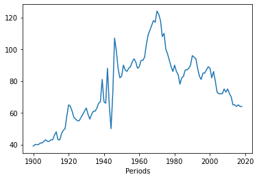
# Now we can plot it, using that same command we used above - plotting a specific value (column) by the index.
# In this case, the index is now the year, which provides a nice little visualization.
df['Marriages_170'].plot()
<AxesSubplot:xlabel='Periods'>
Play around - and some (non-graded) homework
The most important thing is that you start playing around. You don’t need to be able to create beautiful plots or anything fancy, but try to get datasets into a usable format and get some insights!
As an exercise after class, why don’t you try the following:
Find a webpage that has a table on it.
Use the read_html scraper tool we learned above, to scrape the tables and save these to a csv file.
Read the csv file back into python, and try to find some basic descriptive statistics (max, min, mean, etc) and if you can, make a simple visualization out of it (histogram or plot).
Save all of this to a new notebook–code, notes if you have questions or about what you’re doing, and output.
If you can do all of these things, great! If you can’t bring your questions to next class.